

Filming is currently underway on a special online course based on this blog which will include videos, animations and work-throughs to illustrate, in a visual way, how the Fourier Transform works, what all the maths is all about and how it is applied in the real world.
Click here to reserve your free module
The module will be emailed to you the moment the course goes live.
Windowing
In the last post we developed a way of actually calculating the Fourier Transform for real signals. In order to do this, we had to modify all the parts of the Fourier Transform equation that required us to deal with infinite values. This led us to the Discrete Fourier Transform (DFT).
The problem with the DFT is that, by its very nature, it has to be discrete; it skips over some of the information in our signal. This causes additional ghost frequencies to appear in our result. We already saw one way this happens which we called aliasing. In my example signal, which was made up of only 3 frequencies, we discovered that the DFT actually found 6 frequencies in the signal. Luckily aliasing is pretty easy to deal with so long as we ensure that we sample the signal at a high enough rate.
However, this need to be discrete causes another problem, one which is not so easy to deal with. It creates discontinuities at the beginning and end of the signal. The DFT looks at the signal over a non-infinite amount of time, but as the DFT is only a slightly modified version of the Fourier Transform, which expects signals to go on for ever, what does the DFT think happened before the time that the signal began and what does it think will happen after the signal has ended? Have we really solved all our infinity problems simply by changing a few letters in our equation? The answer, of course, is no!
I was very careful when I chose my example signal to demonstrate the DFT in the previous post. You will notice that it is a repeating signal and I allowed it to repeat for 5 whole cycles. This means that if I were to extend the signal for another cycle or another two cycles or even another infinity cycles, there would be no discontinuities at the beginning and end of each cycle. One cycle would flow seamlessly into the next as shown below, the blue line is the signal and the dotted red lines show where one cycle ends and the next one starts.

In the previous post, the number of samples, N, was 40 and my sample rate was 40Hz. This allowed 5 whole cycles of the signal to repeat. What would happen if I decided to make N smaller, say N=35 and perform my DFT on only 35 samples? The signal we were performing the DFT on would look like:

You can see how the 5th cycle is not a complete cycle. If I perform the DFT on this signal then look at the magnitudes of each of the frequencies in my signal I get a graph which looks like:
Frequency Graph when N=35

I am using exactly the same signal as before, I’ve just reduced the amount of the signal I am putting into my DFT. Instead all 40 samples (N=40), I’ve only used 35 (N=35). We can still see the aliasing effect (the non-zero frequency components above 20Hz). We can still see that 5, 10 and 15Hz are the dominant frequencies in our signal, but what is all this noise (all the non-zero values) of all the other frequencies? They were all zero when we performed the DFT on the whole signal (N=40) as shown in the graph below.
Frequency Graph when N=40
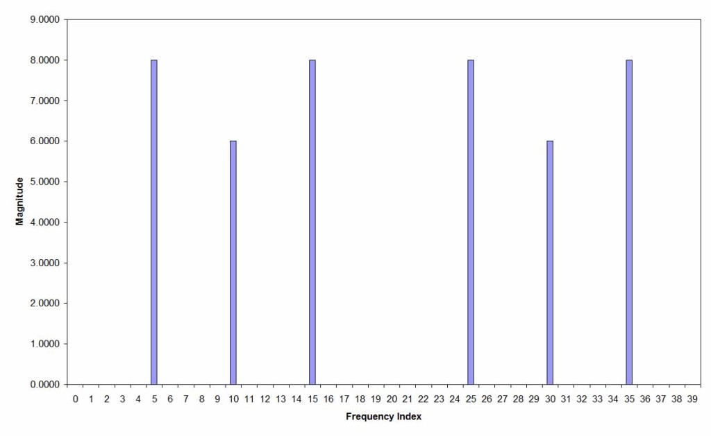
Why, when N=35 does my signal appear to be made up of lots of other frequency components too?
This happens because the DFT assumes that the 35 samples we used at its input are repeating themselves for ever. If I zoom out a little from the actual part of the signal we performed the DFT on, the DFT thinks that the original signal looks like:

To the left of the red dotted line is our original signal. The right of the red dotted line is how the DFT assumes the signal will continue (a straight repeat of the original signal). You can see at this point that there is a discontinuity in the signal. The fifth cycle of the original signal is missing a few samples, but the DFT repeats the signal from the beginning regardless. This is where all those stray frequencies are coming from in our frequency graph when N=35. It is as if the nice sharp peaks of the N=40 graph have leaked into the adjacent frequencies, a phenomenon known as “Spectral Leakage”.
This leakage is going to happen with most real world signals. It’s all very well the DFT assuming that every signal at its input is a repeating signal, but most real world signals do not repeat themselves. Therefore we need some way of coping with this problem.
Unfortunately, we cannot solve it completely, but we can reduce it. The way we reduce it us by a method known as “Windowing”. Windowing takes our signal and fades it in over the first few samples and fades it out over the last few samples. This ensures that the first and last samples in the signal are either zero, or very close to zero (depending on the type of window we use). This greatly reduces the effects of discontinuities in the DFT’s assumed repeating signal which helps to minimize the spectral leakage we saw above.
There are many different types of windowing functions; each is useful for different purposes. I am going to deal with 2 of the most common ones. If, like me, you are a sound engineer, you may have seen these terms as parameters you can change in your spectrum analyzer. Hopefully this next section will help you to understand what it is they actually do.
The Hann Window
The Hann window is named after Julius Ferdinand von Hann, an Austrian meteorologist. It takes the time domain signal and multiplies it by the Hann function:

Where:
w(n) is the windowing function
n is the sample index
N is the number of samples
If N=35, as in the above example, the Hann window w(n) looks like:

If we multiply this by our signal before putting it through the DFT, our signal would look like:

The signal x(n) is shown in blue and the windowing function, w(n) is shown in grey. If we now perform the DFT on this signal, calculate and plot the magnitudes of each frequency on a graph and compare it to the DFT of the non-windowed signal from before:
You can see how the windowing has changed the result. The overall height of the peaks is reduced (this doesn’t matter to us much as it is the relative magnitude of each peak that is of interest), but more importantly there is less noise, more of the in-between frequency components are closer to zero. If we look at what the DFT thinks the repeating signal looks like, we can see why:

At the join between consecutive cycles (shown by the dotted red line) there is no discontinuity, because the Hann window has made sure that the last sample in the first cycle and the first sample in the next cycle are 0. However, we have had to distort the signal quite significantly to achieve that, hence the improved, but still not perfect frequency graph. Unfortunately, this is a problem we are going to have to live with. In order to solve the discontinuity problem, we have to modify the signal. The aim is to modify it in such a way as to improve the accuracy of the frequency domain information as much as possible.
The Hamming Window
The Hamming Window was first proposed by Richard W. Hamming, an American mathematician. It is similar to the Hann window only it never allows the signal to taper off to zero. The Hamming function is given by:

where
0.5 < α < 1.0 – This defines the height of the tail of the Hamming function above zero. For example in the graph below, α = 0.56
β = 1-α
Plotted on a graph, this looks like:

If we multiply this by our signal before putting it through the DFT, our signal would look like:

The signal x(n) is shown in blue and the windowing function, w(n) is shown in grey. If we now perform the DFT on this signal, calculate and plot the magnitudes of each frequency on a graph and compare it to the DFT of the Hann windowed signal from before:

You can see that the results are similar to the Hann window, the peaks are slightly higher though. This is because the Hamming window never fades the signal out completely. There is still a small amount of signal at the beginning and end of the sampled range. This means that there will be a very slight discontinuity where the DFT thinks the signal repeats – where the red dotted line is in the graph below.

Conclusion
So windowing functions don’t get rid of the problem of spectral leakage caused by non-repeating signals, but they do help to reduce it. This is just as well, as most of the useful signals you will encounter in real life are non-repeating. I’ve only covered 2 of the most common windowing functions in this post. You can find more windowing functions here.
So now we can actually perform the Fourier Transform on a real signal and reduce the problems caused by having to finitely sample that signal. However, just in case you thought we were finished, we are left with one more problem. We’re doing a lot of operations with sines and cosines and these functions take quite a bit of computing power to work them out. This might be fine for your PC with its multiple CPU cores and clock speeds in the gigahertz range, but a lot of everyday applications that use the Fourier Transform work on much smaller devices with much less computing power. If only we could achieve the same results for less work. Well, we’re in luck. We’ve spoken a lot in this post about how the Fourier Transform assumes that our signal repeats itself forever. The reason for that is that the sine and cosine waves we are multiplying our signal by repeat themselves forever. This may have caused us a problem in this post, but it is going to be a lot of help next time in the final post in this series when we take a look at the Fast Fourier Transform.

